Experiment 11: CD Diffraction

Purpose: Use laser diffraction to determine the distance between the grooves of a CD.

Materials:

Laser

CD

paper with small hole cut in it

meter stick

stands

clamps

Set Up:

First we needed to find the wavelength of the laser using a simple diffraction experiment. We measured the length (L) from the diffraction grating to the white board. Then we measured the distance (y) from the middle red dot to an adjacent red dot. And the distance between slits on the diffraction grating (d) was given to be 500lines/mm.

Data:

Now we need to caluclate the d between the grooves of a CD by shining the laser on it and using the same equation and wavelength just calculated. By cutting a hole through a piece of paper, we shined the laser through it and the relfection from the laser bounced back and left dots on the backside of the paper. Now we could find y again.

Calculations:

Conclusion:

Our experiment had a 20% error since our measured distance (d) was 1280 nm and the actual distance was 1600 nm. This is a pretty decent result using this procedure, although most of the other groups got a value close to 1600 nm.

Experiment 9: Lenses

Purpose: To observe characteristics of a converging lens and the image it produces from a light source

Materials:

• light source with arrow image
• large converging lens
• lens holder
• meter stick
• marker board
• optics bench

Set up:

Experiment:
1. First we determined the focal length of the lens by using the sun rays outside

f = 5.3

2. Then we took data by changing the distance of the lens from the light source by a factor of the focal length.

Object distance do, cm	Image distance di, cm	Object  height ho,  cm	Image       height    hi, cm	M	Type of      image
5 f = 26.5	7	8.8	2.3	0.26	inverted
4 f = 21.2	7.7	8.8	2.9	0.33	inverted
3 f = 15.9	8.4	8.8	4.6	0.52	inverted
2 f = 10.6	11.5	8.8	9.1	0.96	inverted
1.5 f = 7.95	15.95	8.8	n /a	1.8	inverted

3. Change the object distance to 0.5 f. What happens to the image?
 The image is found inside the lens and is no longer inverted.

If you cannot get an image on the card, take the card away and look through the lens at the object to view the image.  How would you describe the image?  Look through the lens at the object and view the image. How would you describe the image? 

The image is projected as it is seen from the slide of the light source.

4. Plot a graph of image distance, d_i, vs. object distance, d_o using centimeters.

5. Plot a graph of inverse image distance vs. negative inverse object distance.




slope = 0.9037
y-intercept = 0.1748 which represents the minimum image distance the lens will produce.

9.         Using the regression line from your graph and substituting in the axis values, write the equation that relates d_i and d_o below.

Summary: From this experiment we have successfully proved the equation that relates focal length to the object and image distance. p is positive when the object is on the incoming light ray side. q is positive when the image is on the outgoing light ray side.

Experiment 8: Concave and Convex Mirrors

Purpose: To observe the images produced by convex and concave mirrors.

Materials:

• convex mirror
• concave mirror
• marker
• ruler
• worksheets in lab manual

Part A: Convex Mirror

1.         Place an object in front of a convex mirror. Describe the image characteristics as completely as you can.

a)     Does the image appear larger than, smaller than, or the same size as the object?

smaller

b)     Is the image upright or inverted?

upright 

c)      Where is the image located relative to the position of the mirror and object?

 The object image looks closer than the actual object.

2.     Move the object closer to the mirror. Describe the changes in the image. Compare the new image with your answers in Step 1.

The new image just looks very large.

3.            Move the object further from the mirror than it was in Step 1. Describe the changes in the image. Compare the new image with your answers in Step 1. 

The new image appears to be getting smaller.

Calculations:

Part B: Concave Mirror

1.         Place an object in front of a convex mirror. Describe the image characteristics as completely as you can.

a)     Does the image appear larger than, smaller than, or the same size as the object?

larger

b)     Is the image upright or inverted?

inverted 

c)      Where is the image located relative to the position of the mirror and object?

 The object image looks closer than the actual object.

2.     Move the object closer to the mirror. Describe the changes in the image. Compare the new image with your answers in Step 1.

The new image appears very large and very distorted.

3.            Move the object further from the mirror than it was in Step 1. Describe the changes in the image. Compare the new image with your answers in Step 1. 

The new image appeared smaller, inverted, and closer to the image relative to the mirror-object distance.

Calculations:

Conclusion:
The magnification of a concave mirror is negative when the object is far away which makes the image become inverted. For a convex mirror, the magnification is positive since the image produced is upright.

Experiment 7: Introduction to Reflection and Refraction

Purpose: To find a relationship between the angle of incidence and the angle of refraction using a light source.

Materials:

• light box
• semicircular plastic prism
• protractor

Set Up:

 

A cover is placed over the light source to allow only a tiny slit of light to pass through. A plastic prism is laid on top of a protractor. When the prism is rotated the light entering the prism changes the angle it leaves the prism (otherwise known as the angle of refraction). The protractor is used to measure how much the angle changes once it passes through the prism. The angle that the light first hits the prism is known as the angle of incidence. We can find a relationship between the two angles by measuring angle changes in 5 degree increments and graphing the data. The first data table is when the angle of incidence hits the flattened side of the prism and leaves the curved side as shown in the picture above.

Prior to taking data some questions were asked about how the light would behave:

Case 1
light hitting the acrylic straight edge first
incidence angle(θ1)	refraction angle(θ2)	sin (θ1)	sin(θ2)
10	7	0.174	0.122
15	12	0.259	0.208
20	14	0.342	0.242
30	20	0.500	0.342
35	23	0.574	0.391
40	25	0.643	0.423
45	30	0.707	0.500
50	32	0.766	0.530
60	36	0.866	0.588
70	41	0.940	0.656

For this graph a linear fit will sufficiently define the slope of this data.


The slope of this line is the relationship between the two angles. It is called the index of refraction (n). For air the index of refraction is 1 and all values for n are greater than or equal to 1. The slope equation for this line is y = 1.4477x so the index of refraction for this graph is 1.4477.

For part 2 the orientation of the prism was changed:

Case 2 is the data we took for the light hitting the curved side of the prism first and leaving through the straight edge.

light hitting the acrylic with the circular edge first
incidence angle(θ1)	refraction angle(θ2)	sin (θ1)	sin(θ2)
0	0	0	0
5	7	0.087156	0.121869
10	15	0.173648	0.258819
15	24	0.258819	0.406737
20	35	0.34202	0.573576
30	53	0.5	0.798636
40	75	0.642788	0.965926
44	90	0.694658	1

10. Were you able to complete all 10 trials? What happened?

After we reached an angle of incidence of 44 degrees the angle of refraction disappeared.

11. Plot a graph of sin θ₁ vs. sin θ₂ for all the angles you recorded. Determine the regression line and find the slope. What do you think the slope represents? 





12. Using the axis variables, write the equation of this straight line.
 The equation of this line is y = 1.5151x so the index of refraction is 1.5151.

Summary:
The indexes are different but fairly similar in value. This value should be the index of refraction for acrylic. Although there is a measure of uncertainty in the angle values, the data still generated accurate results.

Experiment 6: Electromagnetic Radiation

Purpose: To examine how EM radiation from a simple antenna communicates with a receiver.

Materials:

• copper wire
• leads
• frequency generator
• oscilloscope
• ruler
• BNC adapter

Set Up:

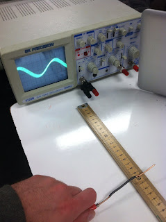
Experiment: The antenna causes disturbances in the wave shown on the screen of the oscilloscope. We needed to find a relationship between the amplitude of the wave on the screen and the distance the antenna was placed from the receiver. We tuned the frequency generator to 30kHz and changed the time and the voltage setting on the oscilloscope until we could see a wave on the screen. We moved the antenna away from the receiver in 5 cm increments and recorded the amplitude of the wave from peak to peak.

We used three tests to make sure what we were doing was influencing the image on the oscilloscope.
1. changing the distance between the metal rod and the oscilloscope
2. changing the voltage on the oscilloscope
3. changing the frequency on the frequency generator

Data:

distance (m)	# of divisions peak to peak	vertical scale	peak to peak amplitude (mV)
0.00	4	50	200
0.05	4	10	40
0.10	2.25	10	22.5
0.15	2	10	20
0.20	1.8	10	18
0.25	3.5	5	17.5
0.30	3.2	5	16
0.35	2.8	5	14
0.40	2.4	5	12
0.45	2	5	10
0.50	1.6	5	8
0.55	1.2	5	6

Trig Variant: We used a A/r and A/r² function to fit the data.

Graph of A/r

Graph of A/r²

The trendline for A/r² does not pass through any of the points so A/r is the best fit between these two graphs.

Graph of A/rⁿ

Summary: Because the transmitter isn't a point charge it sends waves in all different directions so the closer the transmitter it to the receiver  the graph will look more like 1/r. IF the transmitter is far away, then the graph will look more like 1/r².

Experiment 5: Introduction to Sound

Purpose: determine the characteristics of sound waves such as the period, frequency  wavelength, speed, amplitude. Then test variations of its frequencies by having different people speak into the microphone.

Materials:

• Lab Pro microphone
• computer

Experiment:

1. Say “AAAAAAAA” smoothly into the microphone and hit Collect. Once you get a graph that you think is quality, copy it to a Word document and label it #1.  Answer the following questions in your document.

a)      Would you say this is a periodic wave?  Support your answer with characteristics.

b)      How many waves are shown in this sample?  Explain how you determined this number.

c)       Relate how long the probe collected data to something in your everyday experience. For example: “Lunch passes by at a snails pace.” Or “Physics class flies by as fast as a jet by the window.”

d)      What is the period of these waves?  Explain how you determined the period.

e)      What is the frequency of these waves?  Explain how you determined the frequency.

f)       Calculate the wavelength assuming the speed of sound to be 340 m/s. Relate the length of the sound wave to something in the class room.

g)      What is the amplitude of these waves?  Explain how you determined amplitude.

h)      What would be different about the graph if the sample were 10 times as long? How would your answers for the questions a-g change? Explain your thinking. Change the sample rate and test your ideas. Copy the graph and label it #1h.

                                       

2.  Now have someone else in your group say “AAAAAA” into the microphone.  Copy the graph and label it #2.  Compare and contrast the two people’s wave patterns.  Be specific in your answer. For example: determine the characteristics that you did for the first person (# of waves, frequency, period, amplitude, and wavelength) and include any qualitative observations. 

                                                                                

	# of waves	frequency (Hz)	period (s)	amplitude (arbs.)	wavelength (m)
Trial 1	4	154	0.0065	0.7715	2.21
Trial 2	4	125	0.0080	0.7560	2.72

The first trial was a female voice and the second trial was a male voice. The male voice had a lower pitch which accounted  for the lower frequency and larger wavelength.

3.  Collect data for a tuning fork by striking it on a soft object. Copy the graph and label it #3.  Compare and contrast the waves made by human voice.

	# of waves	frequency (Hz)	period (s)	amplitude (arbs.)	wavelength (m)
Trial 1	4	154	0.0065	0.7715	2.21
Trial 3	12	400	0.0025	0.1620	0.85

In the same amount of time collected, the tuning fork made 3 times as more waves as the first person did. The frequency was 3 times as higher and the wavelength was 3 times as smaller.

4.  If you use the same tuning fork to collect data for a sound that is not as loud, what changes would you expect on the display from the sample in #3?  Test your ideas. Copy the graph and label it #4. What did you do to make the sound softer?  Compare and contrast the waves collected for the louder sound.

We tapped it lighter on our hands to make the sounds softer. We expected all the characteristics to be the different.

	# of waves	frequency (Hz)	period (s)	amplitude (arbs.)	wavelength (m)
Trial 3	12	400	0.0025	0.1620	0.85
Trial 4	7	250	0.0040	0.2835	1.36

Everything changed in the softer wave. Since the frequency changed all the other characteristics changed with it.