Experiment 6: Electromagnetic Radiation

Purpose: To examine how EM radiation from a simple antenna communicates with a receiver.

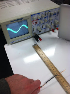
Materials:

• copper wire
• leads
• frequency generator
• oscilloscope
• ruler
• BNC adapter

Set Up:

Experiment: The antenna causes disturbances in the wave shown on the screen of the oscilloscope. We needed to find a relationship between the amplitude of the wave on the screen and the distance the antenna was placed from the receiver. We tuned the frequency generator to 30kHz and changed the time and the voltage setting on the oscilloscope until we could see a wave on the screen. We moved the antenna away from the receiver in 5 cm increments and recorded the amplitude of the wave from peak to peak.

We used three tests to make sure what we were doing was influencing the image on the oscilloscope.
1. changing the distance between the metal rod and the oscilloscope
2. changing the voltage on the oscilloscope
3. changing the frequency on the frequency generator

Data:

distance (m)	# of divisions peak to peak	vertical scale	peak to peak amplitude (mV)
0.00	4	50	200
0.05	4	10	40
0.10	2.25	10	22.5
0.15	2	10	20
0.20	1.8	10	18
0.25	3.5	5	17.5
0.30	3.2	5	16
0.35	2.8	5	14
0.40	2.4	5	12
0.45	2	5	10
0.50	1.6	5	8
0.55	1.2	5	6

Trig Variant: We used a A/r and A/r² function to fit the data.

Graph of A/r

Graph of A/r²

The trendline for A/r² does not pass through any of the points so A/r is the best fit between these two graphs.

Graph of A/rⁿ

Summary: Because the transmitter isn't a point charge it sends waves in all different directions so the closer the transmitter it to the receiver  the graph will look more like 1/r. IF the transmitter is far away, then the graph will look more like 1/r².